Ishan has spent the last two months as an ASIAA summer student with Comet Hunters working on making simulated images of main-belt comets. Ishan has chronciled his progress here and here on the blog. The goal is that with this simulated main-belt comets we can learn about how faint of cometary activity can the project see. This will let us probe the frequencies of main-belt comets in ways we couldn’t do with just the HSC data alone. Thanks Ishan for all your hard work and effort this summer.

Ishan gave his final presentation at the end of August which he is kindly sharing here:

Hello I am Ishan Mishra and my project is ‘Studying Main Belt Comets with Comet Hunters’

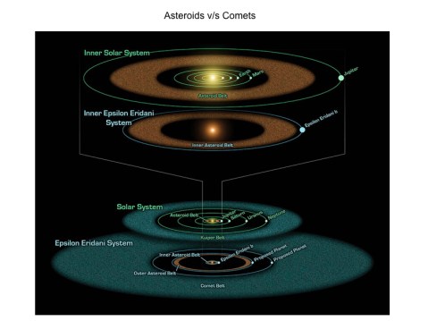Let’s quickly review what are the major differences b/w comets and asteroids:

1. As you can see in this graphic, most of the comets reside in the Kuiper belt beyond the orbit of Neptune and in the Oort Cloud in the outer solar system.
2. The also differ in size and composition. While comets typically range from 6 – 25 miles in diameter, asteroids are much larger with their diameters ranging from the size of small rocks to about 600 miles.
3. Comets contain a lot of ice along with rock and hydrocarbons while asteroids are composed of rocks and metals

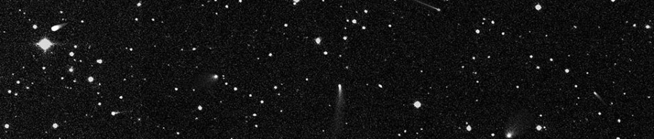
So what are Main-Belt Comets? These are a recently discovered class of main belt objects which show cometary activity. Here’s an image of a main belt comet taken by the Subaru Telescope.

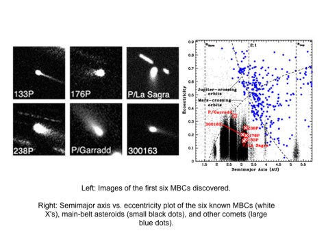Here we see images of the first six MBCs discovered. The plot on the right clearly shows that these objects are distinct from comets while being indistinguishable from asteroids.

So why are we interested in MBCs?

1. Firstly, our classic difference between asteroids and comets based on their composition is called into question. Asteroids were never known to have volatiles present in them.

2. Present-day sublimation in the main belt is surprising, as surface ice is unsustainable over the age of the Solar System so close to the Sun. MBCs provide new constraints to the location of the so-called snow-line (the distance from the Sun beyond which primordial temperatures in the protoplanetary disk were low enough for water to condense as ice and thus be swept up into forming planetesimals)

3. The astrobiological implication: Origin of water on Earth. This interests me the most!

The Earth is believed to have formed dry owing to its location inside the snow line, and therefore the water we see today must have been delivered from outside the snow line, perhaps by impacting asteroids and comets. There are models which suggest that water delivery from asteroid belt was more likely. MBCS provide us a way to test this.

However, so far very few MBCs, about 12, have been discovered. We need to find more in order to:

1. Determine their extent and abundance
2. Having a large dataset will help us understand them better

The search efforts so far have been mainly of two kinds: Using computer based pattern recognition algorithms and using human pattern recognition abilities.

1. Computer algorithms currently are not faring well because of the very low SNR of the coma/tail region. They are also unable to accurately account for the whole range of tail morphologies. Hence, there are a lot of false positives.

2. Telescopic surveys provide the large datasets needed to increase chances of finding objects like MBCs. PAN-STARRS is one such survey which uses a 2 m telescope in Hawaii. Here is an image of the first MBC discovered using PAN-STARS dataset. There are a couple of issues with this method though:

1. The image quality is not good as its a small telescope. In fast, most surveys use a small telescope.
2. Since the search is conducted by eye and the team consists of just a few scientists, the process is very slow and laborious.

Here’s where Comet Hunters comes in as a possible savior.

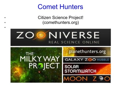So, Comet Hunters is a Citizen Science project under the citizen science web portal called Zooniverse. The idea behind citizen science is crowdsourced scientific research, ie, a large number of volunteers, their numbers usually in thousands, actively participating to complete research tasks.

Projects at Zooniverse span Astronomy, Climate Science, Biology, Physics and even Humanities. Galaxy Zoo is a famous example of astronomy related. The volunteers are shown images of galaxies and they have to classify them according to their morphologies. Another is Planet Hunters, where you need to spot dips in light curves corresponding to planet transition.

In Comet Hunters, volunteers are shown images of asteroids and they need to check for the presence of a coma or a tail. A candidate is vetted by the research team only when about 20 volunteers spot any activity. The combined assessments of so many people are much more reliable than individual opinions.

1. So we have a large number of searchers now. What about the data?

The data for Comet Hunters comes from Subaru, an 8 m telescope at Mauna Kea, Hawaii.

Two key advantages:

1. Large telescopes are rarely used for surveys. So we have a large amount of high quality data.
2. Two catalogs: Suprime Cam Archive and the Hyper Suprime Cam current survey data. So we have 17 years worth of data. Easier to spot recurrent activity.

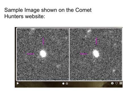Here’s a just a quick example of an image shown on the Comet Hunters website.

It can be also be seen with inverted colors for more clarity.

The two images are about 20 arcsec in width each and are from the same night.

The volunteers need to answer whether a tail is present in one image, both images or is completely absent.

1. We have a large number of people now working on high quality data. But,

What is the detection efficiency of Comet Hunters? How good is the project in detecting MBCs? What kind of MBCs are getting detected?

This where my project comes in.

My job is to create or simulate asteroid images similar to Subaru’s, with varying properties like the coma or tail strength, tail direction, etc.

The volunteers’ choices for these images will help us characterize the kind of MBCs that are being detected by Comet Hunters. For example, we can find the minimum strength of the coma/tail for which the volunteers are able to spot them.

Here are a two examples of images that I have generated till now. I will explain the process in the subsequent slides.

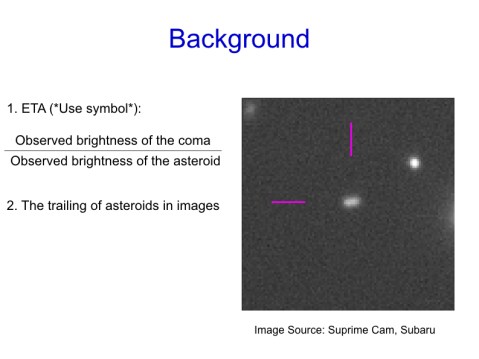
Before I start talking about my work, I need to give some background information.

1. I will be using this term called ETA to denote the strength of coma activity. As you can see, a value of 0 means absence of coma.

2. If you look closely in the Subaru images, you will find that the asteroid image is elliptical not circular. I exaggerated the stretching in the model images I displayed in the previous slide. And you can also see this in on the image on left.

So why does this happen?

Solar system objects move much faster in the plane of sky than the distant stars. And Subaru’s survey data images are usually taken for exposure times of 120-150 seconds, as they are not specifically designed for solar system observation.

So during this interval the asteroids/comets move a couple of arcsec resulting in smearing or stretching of the image in the direction of motion.

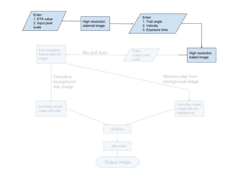
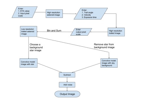
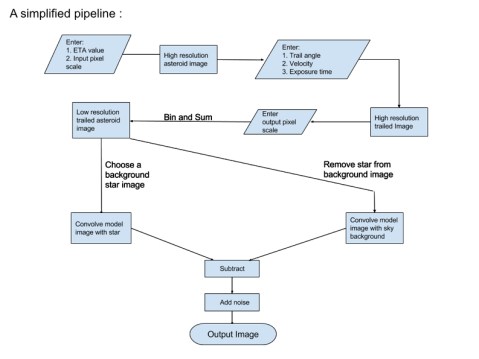Here I present a simplified pipeline for the generation of model MBC images. As you can see, there are a lot of steps involved. Let’s go through them one at a time.

1. The first part is the generation of a simple asteroid image with or without a coma, whose intensity strength we can control.
2. The second box says high resolution asteroid image. This means that we are starting with images at a much higher resolution than that of images obtained from Subaru. I will come to the reason shortly. (*Planning to talk about it when I explain bin and sum*)

Let’s see how a simple asteroid looks.

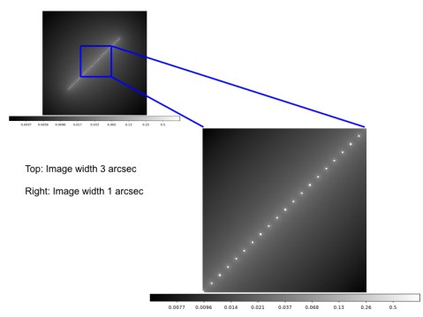
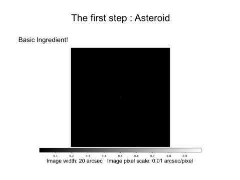Here is our asteroid, just a pixel wide, with no coma. So, all the pixels in this image have value zero except the central pixel which has the value 1.0.

2. This is how the asteroid will look if we see it in space, without any optical or atmospheric effect. The ideal case.
3. The image is 20 arcsec in width with a resolution of 0.01 arcsec per pixel (compared to Subaru’s resolution which is approx. 0.17 arcsec per pixel).
4. Let’s zoom in to the central 1 arcsec region to see the asteroid clearly

So we see a tiny dot at the center which represents the asteroid.

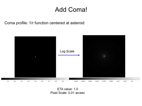
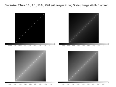
1. Now let’s add a coma to the asteroid. If you remember, we defined a parameter ETA which is proportional to the intensity strength of the coma. Here you see an asteroid with a coma of intensity 1.0
2. The coma is invisible in the default linear scale image. So I have also shown the log scale image to confirm the presence of a coma.

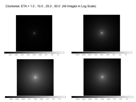
1. Here are some images of asteroid with coma of different intensities. The ETA increases clockwise. Again, these images are all in log scale for clarity.

So, we have our asteroid image with a coma around it. Let’s move on to the next stage.

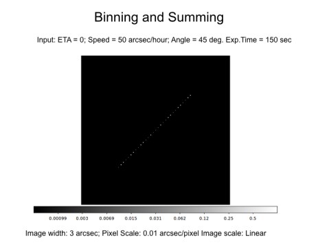
1. We now trail the asteroid. As I had mentioned earlier, trailing is necessary to account for the stretched asteroid image which is due to the significant movement of asteroid in sky during the telescope exposure time.

2. The information we need to trail the asteroid is its speed and direction of movement as seen in the plane of the sky and the exposure time of the telescope, which will control the length of the trailed image.

Let’s see an example.

1. Here I trail an asteroid with coma of ETA value 25.0. We trail it with a speed of 50 arcsec/hour, at an angle of 45 degrees for an exposure time of 60 seconds.

2. I have purposely shown the asteroid image in linear scale so that we can see the difference in the background intensity between the two images. Naturally, the comae from adjacent asteroids add up in the second image to make it look brighter.

Let’s zoom in.

1. We zoom into the central 1 arcsec region and now we can clearly see the individual asteroid replicas.

2. The gap between successive asteroids is because we are imaging in an interval of 0.5 seconds for the duration of exposure. Hence, the asteroid is displaced by the distance it moves in this small interval.

Just a quick look at the trailed asteroid images for different coma intensities. All these images are of the central 1 arcsec region and are shown in logscale.

OK. Now that we have the trailed asteroid, we proceed to a very important step: Reducing the resolution or increasing the pixel scale to Subaru’s.

A look at the trailed asteroid images for different trailing directions

1. So in this step we go concert our high resolution images, of pixel scale 0.01 arcsec/pixel, to the lower Subaru resolution of 0.17 arcsec per pixel. But why did we start with a higher resolution?

2. We are starting with how the image looks from space, before passing through the asteroid and being images by the CCD in the telescope. This is why we started with a single pixel wide asteroid, a point source.

3. So, we are basically replicating how a CCD works, with all the photons falling in a square CCD pixel account for its value.

1. So in this step we go concert our high resolution images, of pixel scale 0.01 arcsec/pixel, to the lower Subaru resolution of 0.17 arcsec per pixel. But why did we start with a higher resolution?

2. We are starting with how the image looks from space, before passing through the asteroid and being images by the CCD in the telescope. This is why we started with a single pixel wide asteroid, a point source.

3. So, we are basically replicating how a CCD works, with all the photons falling in a square CCD pixel account for its value.

Here’s a practical example: the famous Eagle nebula.

Before we proceed, I would like to mention that prior to using this binning and summing technique to decrease resolution, we were trying to use interpolation. It didn’t work out at the end as we discovered a major flaw with the method or maybe the interpolation function we were using wasn’t working as expected. We can talk about this later if anyone’s interested.

OK. So let’s see how the low resolution images of our trailed asteroid look.

Here’s a high resolution trailed image that we saw before. The input parameters are also shown. As you can see, this one has ETA = 0 , ie , no coma.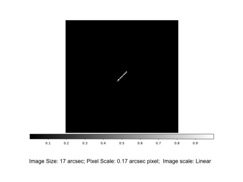This is the low resolution image. It is 101 x 101 pixels wide. Please note that I have verified the total flux (in this case the sum of all pixel values) is conserved during the sum and bin process.

Here are some more low resolution image with same parameters as the previous image except ETA.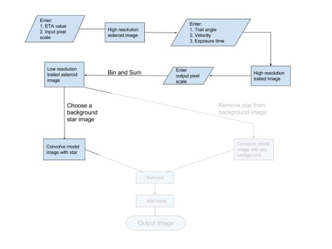OK. Let’s move on now to the final stage: convolving our model asteroid with a background star. But why do we need this?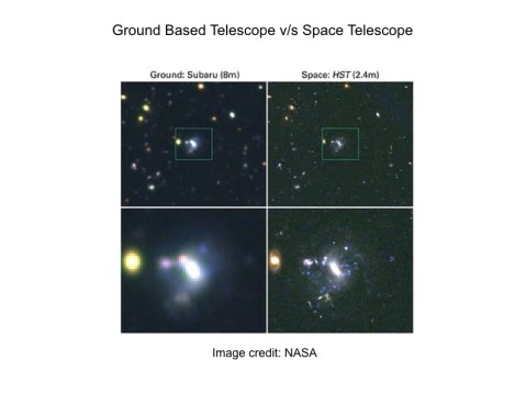To account for two things that affect the ideal image: Atmosphere and Telescope optics. Convolving with a background star incorporates these effects into our ideal image and makes it looks realistic. 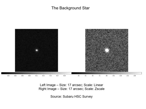Here’s the background star which we will use for the convolution process. This was chosen by eye from a field image obtained from HSC database.

You will notice that the image on the right here and many subsequent images are shown in zscale. This is because the Subaru images fed into the CometHunters website are in zscale. This scaling provides a convenient perspective to look for any activity in the object.

Let’s see how our convolution process fares for some model images we have seen so far.

Case 1: The most basic one: untrailed asteroid with no coma.

As you see, since the model asteroid in this case is basically a delta function, the background star image is identically reproduced.

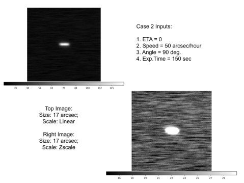
Case 2: Horizontally trailed coma asteroid with no coma.

Now here we encounter a major problem. The noisy background from the star’s image is getting trailed in the direction of asteroid’s movement. We have been trying to remedy this by playing with the convolution process but to no avail.

Recently, we came up with a neat trick. Why not generate a trailed sky background image same as in the convolved output but without the central asteroid. Then, ideally, subtracting this trailed background with our convolved output should remove the background from the latter image, leaving just the asteroid part we are interested in.

Let’s see how this works.

Firstly, to generate the sky background we need to convolve our model asteroid with the background image (with star removed). We remove the star from the background image by simply replacing a central square region containing the star (the image on slide 31) with some random background sky region. This process is crude and not the best way to remove the star, but will have to work for now.

You can see that the background sky gets trailed when convolved, as expected.

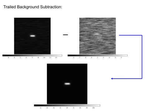
Now we subtract our convolved output (from slide 33) with our trailed background image from the previous slide and…..Voila! The background gets removed perfectly!

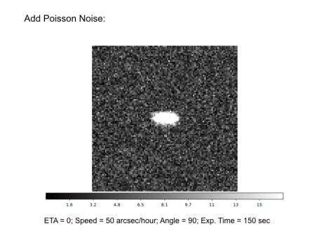
Now the final step is to add noise in this image. We add poisson noise to each pixel because of something called shot noise.

Shot noise is caused by the random arrival of photons.  This is a fundamental trait of light.  Since each photon is an independent event, the arrival of any given photon at a pixel cannot be precisely predicted; instead the probability of its arrival in a given time period is governed by a Poisson distribution.

Slide 38:

Here you look at our final output image. Looks good, doesn’t it?!

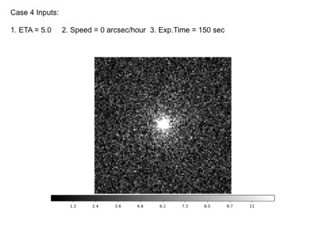
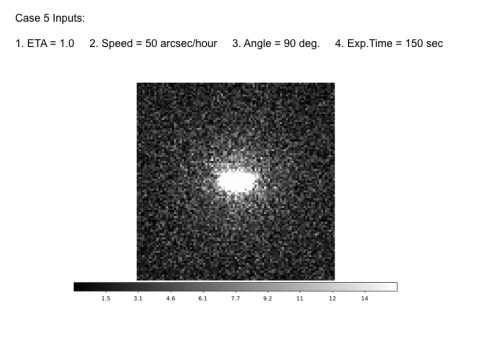
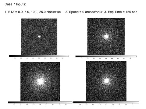
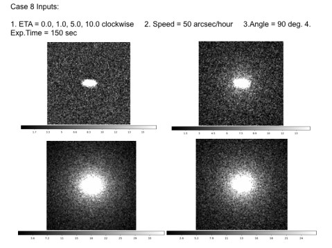
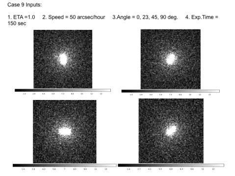
Some sample cases

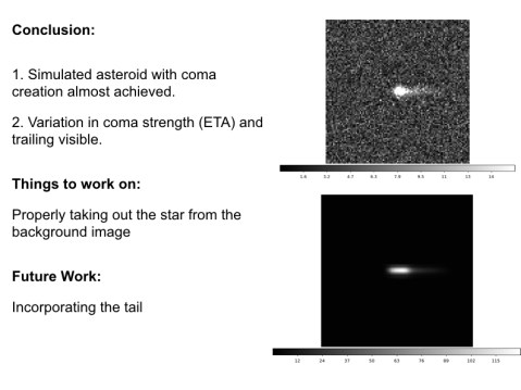
Conclusion and Future work.
Although the pipeline is not completely ready to generate a the complete range of images of asteroids with tail, I quickly generated a basic asteroid with tail image – a pixel wide asteroid at center with a horizontal tail with intensity going of as 1/r – and fed it to the pipeline. The two images on the right depict asteroids with tails. Not bad, eh?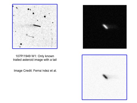

The image on the left is the only recorded image in literature of a trailed asteroid with a tail – 107P/1949 W1. This is an old image, on photographic plate.

On the right hand side I am showing you something similar that I tried to generate from my pipeline. The image on right hand side top is in a linear scale image while the one on the right bottom is the inverse color version, just like the 107P/1949 W1 image on left hand side.